Documentation and Methods

Documentation and methods are organized in the following sections:

• Overview
• How These Estimates Differ From Other ERS Productivity Accounts for the United States
• Model
• Data Sources
  • Outputs
  • Inputs
  • Quality-adjusted Agricultural Land
  • Input Cost Shares
• Country and Regional Productivity
• Suggested Citation

See Summary Findings and details for the Update and Revision History. References are also available.

Overview

Improving agricultural productivity has been the world's primary means of assuring that the needs of a growing population don't outstrip the ability to supply food. Over the past 50 years, productivity growth in agriculture has allowed food to become more abundant and cheaper (see New Evidence Points to Robust But Uneven Productivity Growth in Global Agriculture, Amber Waves, September 2012). One of the most informative measures of agricultural performance and productivity is total factor productivity (TFP). TFP takes into account all of the land, labor, capital, and material resources employed in farm production and compares them with the total gross output of crop, animal and aquaculture products. If total output is growing faster than total inputs, we call this an improvement in total factor productivity ("factor" = input). TFP differs from measures like crop yield per acre or agricultural value-added per worker because it takes into account a broader set of inputs used in production. TFP encompasses the average productivity of all of these inputs employed in the production of all farm commodities.

"Growth accounting" provides a practicable way of measuring changes in agricultural TFP over time given available data on agricultural outputs, inputs, and their prices. The approach described here gives internationally consistent and comparable agricultural TFP growth rates, but not TFP levels. Most of the data on production and input quantities used in this analysis come from UN agencies, especially FAOSTAT database of the Food and Agriculture Organization (FAO) and ILOSTAT labor statistics from the International Labor Organization (ILO). These data are supplemented with data from national and other statistical sources as well as published studies on agricultural productivity. Other data sources consulted include the USDA National Agricultural Statistical Service, USDA Foreign Agricultural Service PS&D database, EUROSTAT, National Bureau of Statistics of China, the Indonesia Badan Pusat Statistik, Statistics New Zealand, IFASTAT of the International Fertilizer Association, and the GGDC Structural Change databases produced by the University of Groningen Growth and Development Center (Timmer et al., 2015; de Vries et al., 2021).

How These Estimates Differ From Other ERS Productivity Accounts for the United States

To facilitate international comparisons in ERS International Agricultural Productivity (IAP) data product, certain simplifying assumptions must be made. As such, the estimates of TFP growth reported here may differ from TFP growth estimates reported in other studies using different assumptions, data sources, or methods. In particular, the TFP estimates reported in IAP data product for the United States differ somewhat from those reported in the ERS Agricultural Productivity in the U.S. data product. The principal differences are (i) the Agricultural Productivity in the U.S. data product excludes aquaculture from output measurement and uses prices received by U.S. farmers (where subsidies are added and indirect taxes are subtracted from market values) for constructing revenue shares and measuring output growth, whereas the IAP data product uses global average agricultural prices to aggregate output; (ii) in the Agricultural Productivity in the U.S. data product, agricultural labor is quality-adjusted by labor’s demographic characteristics—including sex, age, educational attainment, and employment class, whereas the IAP data product uses a headcount of agricultural labor unadjusted for quality differences; (iii) the Agricultural Productivity in the U.S. data product uses a more refined measured of agricultural capital stock in which structures and machinery are assumed to have different rates of depreciation, whereas the IPA data product uses an FAO measure of agricultural capital stock that treats all forms of capital as having a similar rate of depreciation; and (iv) the Agricultural Productivity in the U.S. data product has greater detail on trends in use of intermediate inputs (such as fertilizers, feeds, pesticides, seeds, energy, and purchased services), while the IAP data product has only two categories of intermediate inputs—one for crops based on fertilizer inputs and one for animals and fish based on feed inputs. Generally, the TFP index reported in the Agricultural Productivity in the U.S. data product should provide a more accurate measure of the rate of technical change in U.S. agriculture. However, the IAP data product is better suited for making comparisons of agricultural TFP growth between the United States and other countries.

Model

Total factor productivity (TFP) is defined as the ratio of total output to total inputs. Let total output be given by Y and total inputs by X. Then TFP is simply:

(1)

It is often difficult to provide meaningful definitions of real output or real input due to the heterogeneity of outputs produced and inputs used. However, it is possible to provide meaningful definitions of output growth and input growth between any two periods of time using index number theory (Caves, Christensen and Diewert, 1982). Changes in TFP over time are found by comparing the rate of change in total output with the rate of change in total input. Expressed as logarithms, changes in equation (1) over time can be written as

(2)

which simply states that the rate of change in TFP is the difference between the rate of change in aggregate output and input.

Agriculture is a multi-output, multi-input production process, so Y and X are vectors. When markets are in competitive equilibrium and the underlying technology is represented by a constant-returns-to-scale production function, then output elasticity with respect to an input equals the cost share of that input. Then equation (2) can be written as

(3)

where R_i is the revenue share of the ith output and S_j is the cost-share of the jth input. Total output growth is estimated by summing over the growth rates for each output commodity weighted by its revenue share. Similarly, total input growth is found by summing the growth rate of each input, weighted by its cost share. TFP growth in Eq. (3) is thus the value-share-weighted difference between total output growth and total input growth. The growth rates are then used to construct an annual index from a base year where the index is assigned a value of 100. Index values in a particular year reflect the percentage change in the value of the series between the present year and the base year.

One difference among index number methods is whether the revenue and cost share weights are fixed or vary over time. Paasche and Laspeyres indices use fixed weights whereas the Tornqvist-Thiel and other chained indices use variable weights. Allowing the weights to vary reduces potential "index number bias." Index number bias arises when producers substitute among outputs and inputs depending on their relative profitability or cost. In other words, the growth rates in Y_i and X_j are not independent of changes in R_i and S_j. For example, if labor wages rise relative to the cost of capital, producers are likely to substitute more capital for labor, thereby reducing the growth rate in labor and increasing it for capital. In agriculture, cost shares of agricultural capital and material inputs tend to rise in the process of economic development while the cost share of labor tends to fall.

In the IAP data product, cost shares are varied by decade whenever such information is available. This reduces potential index number bias in the measure of aggregate input change over time. For outputs, base year prices (or equivalently, base year revenue shares) are fixed, since these depend on FAO’s measure of constant, gross agricultural output (described in more detail below in the Outputs subsection under Data). The base period which FAO uses to construct average output prices is 2014–16.

Cost shares are assembled from published studies of agricultural productivity for specific countries and regions, but are not available for all 179 countries and territories in the IAP data product. When cost shares are not directly observed for a country, they are inferred from cost shares of a similar country (a nearby country with a similar agricultural structure and level of economic development). Direct estimates of cost shares were assembled for 22 countries from 17 studies. These 22 countries account for about two-thirds of world agricultural output. For another set of countries or regions where input prices are not available or market-determined, (Sub-Saharan Africa and transition economies of the former Soviet Union and Eastern Europe), three studies provide econometric estimates of production elasticities, which were used in place of cost shares. These regions account for another 8 percent of world agricultural output. For remaining countries, representing about 25 percent of world agricultural output, cost shares are approximated by applying cost shares from a similar country. The section below on Input Cost Shares provides details on the data sources and assumptions.

The framework outlined above provides a simple means of decomposing the relative contribution of TFP and inputs to the growth in output. Using the function g(^.) to signify the annual rate of growth in a variable, the growth in output is simply the growth in TFP plus the growth rates of the inputs times their respective cost shares:

(4)

Equation (4) is a cost decomposition of output growth since each S_jg(X_j) term gives the growth in cost from using more of the jth input to increase output (holding prices fixed). It is also possible to focus on a particular input, say land (which we designate as X₁), and decompose growth into the component due to expansion in this resource and the yield of this resource:

(5)

This decomposition corresponds to what is commonly referred to as extensification (land expansion) and intensification (land yield growth). We can further decompose yield growth into the share due to TFP and the share due to using other inputs more intensively per unit of land:

(6)

Equation (6) is a resource decomposition of growth since it focuses on the quantity change of a physical resource (land) rather than its contribution to changes in cost of production.

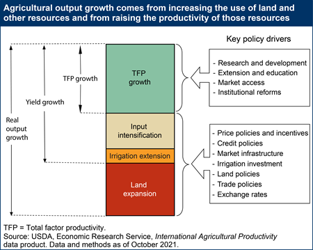
The figure below gives a graphical depiction of the growth decomposition described in equation (6). The height of the bars indicate the growth rate of real output. Growth in real output is first decomposed into growth attributable to agricultural land expansion (extensification) and growth attributable to raising yield per hectare (intensification). Next, yield growth itself is decomposed into input intensification (i.e., more capital, labor and fertilizer per hectare of land), extension of irrigation to existing cropland (which can raise cropping intensity and yield per crop) and TFP growth, where TFP reflects the efficiency with which all inputs are transformed into outputs. Improvements in TFP are driven by technological change, improved technical and allocative efficiency in resource use, and scale economies. Growth in factor inputs is driven by  input and output prices and terms of trade. The decomposition of output growth into the components depicted in the figure is both intuitively appealing and has direct policy relevance: land expansion and input intensification are strongly influenced by changes in resource endowments and prices, whereas TFP growth is strongly influenced by long-term investments in agricultural research and extension services, education, and infrastructure, and improved resource quality and institutions.

Data Sources

FAO’s annual time series of crop, livestock and aquaculture commodity outputs and land, capital, fertilizer and animal feed inputs, and ILO estimates of agricultural labor are the primary data used to construct the national, regional and global quantity measures. In some cases these are modified or supplemented with data from other sources when they are considered to be more accurate or up-to-date, as described below. Other data sources include national statistical agencies, EUROSTAT, the National Statistical Bureau of China, the United States Department of Agriculture’s National Agricultural Statistical Service and Foreign Agricultural Service’s PS&D database, and the Groningen Growth and Development Center (GGDC). The TFP estimates use the latest available data from these sources. These sources sometimes revise data from previous years to reflect more complete information on these series. Updates to the ERS International Agricultural Productivity database include these revisions to previous years’ data from these sources.

Outputs

Agricultural output consists of quantities harvested of 162 crops, 30 animal products, and 8 aquaculture products, for a total of 200 commodities. For the crop and animal outputs, FAOSTAT publishes estimates of annual production by country since 1961. Aquaculture products are from FAO's FISHSTAT. These outputs consist of food and non-food commodities, but exclude harvested hay and fodder and most ornamental crops like flowers and shrubberies.

These 200 farm outputs are aggregated using global average prices from 2014–16 (in purchasing-power-parity dollars) into a measure of the gross value of agricultural output. For crop and animal outputs, the set of global average prices are derived from the FAOSTAT measure of the Value of Agricultural Production. Dividing this measure by the gross quantity produced provides the average unit value or price in $/metric ton for each commodity. The set of common commodity prices is derived by FAO using the Geary-Khamis method (Rao, 1993). For aquaculture products, FISHSTAT provides estimates of gross quantity and value (in current U.S. dollars) for 8 categories of products harvested from aquaculture farms. Dividing global total value by quantity gives the average unit value ($/metric ton) of each product group. These are averaged over 2014–16. For each country or territory, the total gross value of agricultural output in each year since 1961 is estimated taking the annual production quantity times the 2014–16 global average set of commodity prices. For exposition purposes, this output measure is reported as "constant 2015 international dollars" or "dollars as constant 2015 prices." Since constant end-period prices are used to construct the output measure, it is equivalent to a Paasche quantity index of real output.

This measure of agricultural output differs from commonly used agricultural value-added or agricultural GDP reported in national accounts in two important ways. First, agricultural value-added or GDP uses current national prices to aggregate commodities. Second, agricultural value-added subtracts the value of intermediate inputs, such as seed, feed and fertilizers. The agricultural value-added or GDP output measure is useful for measuring agriculture’s share of a national economy. However, agricultural GDP can provide a distorted measure of real output growth over time and across countries. If agricultural GDP is deflated by a national price index, changes in "constant agricultural GDP" will be influenced by terms of trade effects (i.e., when agricultural commodity prices change at a different rate then the general rate of inflation). International comparisons of agricultural GDP will also be affected by exchange rate distortions and differences in national agricultural prices affected by national agricultural policies. For international comparisons of the real volume and growth of agricultural output over time, the measure used here (using global average prices from 2014–16) avoids these distortions.

For the 15 countries of the former Soviet Union (FSU), FAOSTAT reports crop and animal outputs from 1991 onward, and only for FSU as a whole from 1961 to 1990. To derive time series of crop and animal outputs for these countries, historical data on quantities of major crop and livestock commodities were collected. Shend (1993) provides detailed estimates of agricultural output by commodity for each Soviet Socialist Republic (SSR) from 1980 to 1995, and Lerman et al. (2003) provide additional data for each SSR starting from 1965. For some minor commodities and for all commodities for 1961–64, FSU production totals were allocated to each SSR based on their proportion of national production in the most recent year for which SSR data are available.

Inputs

The index of total agricultural input is an aggregation of the quantity of labor, land, capital, and intermediate inputs employed in agricultural production. For labor, land, and capital, annual service flows from "stock" quantities of these inputs are combined with annual expenditures on both farm-supplied and purchased intermediate inputs, divided into six categories: labor, agricultural land, two forms of capital inputs (farm machinery and livestock), and two types of intermediate inputs (inorganic fertilizers and animal feed). The primary source of information is FAO, which published annual estimates beginning in 1961 for each country (except for countries created since that time, such as countries that made up the former Soviet Union, Yugoslavia, Czechoslovakia, Ethiopia and Sudan). For countries created after 1961, the TFP series begins at the time of independence, except for countries of the former Soviet Union, for which time series have been extended back to 1961 using data from Shend (1993) and Lerman et al. (2003).

Agricultural Labor

Agricultural labor is the total number of adults (males and females) whose main economic activity is agriculture. It includes hired labor and unpaid family labor, full time and part time workers, but may exclude some seasonal workers whose main occupations are non-agricultural.

Several sources were consulted for historical estimates of agricultural labor, and the labor data used for the international productivity accounts is a composite of several sources:

1. For most developing countries and countries of the former Soviet Union, the principal data source for agricultural labor is the ILOSTAT modeled estimates of agricultural labor for 1991 and onward. These estimates are back cast to 1961 using growth rates from other sources, especially previously published from FAOSTAT or estimates from GGDC. For former states of the Soviet Union, pre-1991 estimates are from Lerman et al. (2003).
2. For most developed countries, ILOSTAT survey estimates or EUROSTAT survey estimates of agricultural labor are used.
3. For some countries, ILOSTAT estimates appeared to be drawn from incomplete or inconsistent surveys, such as surveys covering only urban or male workers. For these countries, alternative sources are used to construct historical data. These include:
   1. China (source: National Bureau of Statistics of China)
   2. Egypt (source: Fuglie et al., 2021)
   3. South Africa (source: Liebenberg, 2012)
   4. Ireland (source: Matthews, 2000)

Agricultural capital

Agricultural capital are inputs that are used over the course of several seasons or years. Reproducible capital consists of farm machinery and implements, buildings and structures, fruit and nut-bearing trees, and breeding stock. Sometimes land (nonreproducible capital) is also included in measures of agricultural capital. Here, agricultural capital is restricted to reproducible capital and land is treated as a separate category of agricultural input. Generally, reproducible capital inputs are most productive when new and become less productive as they age. Eventually they are scrapped and replaced.

Agricultural capital stock from 1995 to 2020 is from FAOSTAT. FAO constructs capital stock using the perpetual inventory method (PIM), wherein the past 25 years of spending on capital goods (not including land purchases) is aggregated, with older capital loosing efficiency by a depreciation rate of 6 percent per year (Vander Donckt et al., 2021). Thus, to construct its capital stock series FAO requires data on capital investment since 1970 (since the 1995 capital stock is an aggregation of capital investment from 1970 to 1994). Capital investment is taken from national economic accounts. For years in which capital investment data are missing, FAO assumes capital investment is given fraction of agricultural output (the agricultural investment ratio, or AIR). AIR is derived from a statistical model of country characteristics, varying by country and over time according to these characteristics (see Vander Donckt et al., 2021).

To estimate agricultural capital stock from 1961 to 1994, we aggregate the inventories of agricultural machinery and animals held on farms and use the growth rate in these capital goods to back cast the FAOSTAT stock measure for these years. Data users should thus be aware that the agricultural capital stock measure combines two methods for capital stock aggregation: the current inventory method for 1961–94 and the perpetual inventory method for 1995–2020. The current inventory method may be less robust than the perpetual inventory method because (i) it does not take into account capital depreciation and (ii) it does not include all types of capital goods (consisting of only farm machinery and breeding stock). However, because of limited historical information on capital investment for many countries, this is the only available means for deriving a long-term time series for global agricultural capital stock that is comparable across countries and regions.

Animal inventories is the aggregate number of animals used for breeding, milking, egg laying, wool production, and to provide animal traction. To approximate livestock capital, total inventories of animals on farms, measured in "cattle equivalents" are used. Inventories include dairy cows, other cattle, water buffalo, camels, horses, other equine species (asses, mules, and hinnies), small ruminants (sheep and goats), pigs, and poultry species (chickens, ducks, and turkeys), with each species weighted by its relative size (see Table 1).

Farm machinery is the total metric horse-power (CV) of major farm equipment in use. It is the aggregation of the number of 4-wheel riding tractors, 2-wheel pedestrian tractors, power harvester-threshers, and milking machines. Table 1 shows the average CV per machinery type assumed for aggregation purposes. Due to insufficient information no adjustment is made for differences across countries or over time in farm machinery sizes within these categories, except for China, which reports farm machinery inventories in power units (National Statistical Bureau of China). Also, for Indonesia, the FAO estimate of the number of power thresher-harvesters in use includes both pedal and power threshing machines. We include only power thresher-harvesters from Indonesian national statistics, as reported in Fuglie (2010).

Table 1. Weights used to aggregate machinery and animal inventories

Machinery	Weight (CV/unit)
4-wheel tractor	40
2-wheel tractor	12
Harvester-thresher	20
Milking machine	1
Animals	Weight (per head)
Non-dairy cattle	1.00
Dairy cows, buffalo, horses	1.25
Camels	1.38
Asses, mules, other camelids	1.00
Pigs	0.25
Goats and sheep	0.13
Poultry species	0.0125
Note: CV=metric horsepower. Machinery weights are own estimates; livestock weights are from Hayami and Ruttan (1985, p. 450).

FAOSTAT reports continuous time series data through 2009 for the number of 4-wheel tractors, harvest-threshers and milking machines in use, but it does not report numbers for 2-wheel walking tractors. For many developing countries, particularly in Asia, 2-wheel tractors have been a major component of farm mechanization. For 2-wheel tractors, FAO reports numbers in use for 1970s but then discontinued this series until recommencing it in 2002. For interim years, national farm machinery statistics were collected on 2-wheel tractors in use from the agricultural censuses of China, Japan, South Korea, Taiwan, Thailand, Philippines, Indonesia, Indian, Bangladesh, Pakistan, and Sri Lanka, and interpolated between census years. These countries constitute most of the global use of 2-wheel tractors on farms.

Although livestock and machinery inventories are only used to estimate agricultural capital stock over 1961 to 1994, the ERS IAP data product continues to report these series through 2020. For estimates of farm machinery inventories since 2009, estimates are compiled from national statistical sources, market data on new machinery sales, and from modeled projections.

To extend estimates of farm machinery to 2020, national statistics on the number of tractors and combine-harvested from more recent years were collected for a number of countries: Bangladesh (Hassan, 2013), China (National Statistical Bureau of China), Europe (Eurostat), India (Singh et al., 2015), Japan (Ministry of Agriculture, Forestry and Fisheries), Russia (Russian Federation Federal State Statistics Service), and the United States (USDA National Agricultural Statistical Service).

To extend estimates of farm machinery stocks held on farms beyond the last available census or survey estimate, two approaches were used. The first approach uses annual data on new machinery sales, taking into account obsolescence of older machinery, assuming a 15-year useful lifespan for new farm machinery. Data on annual sales of new farm tractors and combine-harvesters during 1991–2020 were collected from farm machinery manufacturers (sources: VDMA, Verband Deutscher Maschinen- und Anlagenbau, or the Mechanical Engineering Industry Association, and Deere corporate reports) for the United States, Canada, Brazil, Argentina, Mexico, South Africa, and European countries. Estimates of farm-held machinery stocks were extended from the latest available census year by adding the number of new machinery sales since the census year and subtracting the number of tractors purchased 15 years earlier. In other words, if M_c is the stock of machines held on farms in census year c, then the number estimated to be held on farms in year c+1 is:

(7)

where S_c+1 is the number of new machinery sales in year c+1 and S_c+1-15 is the number of sales 15 years prior to year c+1. Farm machinery stock in year c+2 is estimated as M_c+2 = M_c+1 + S_c+2 – S_c+2-15, and so on for subsequent years. Individual types of farm machinery were then aggregated into the total stock of metric horsepower held on farms using the machinery weights in Table 1.

The second approach, used for countries for which we do not have information on annual machinery sales, uses an econometric model to estimate the change in farm-held machinery stocks over time since the latest available data on farm machinery stocks. The econometric model is based on the Kislev-Peterson model of farm machinery adoption and farm size. Kislev and Peterson (1982) hypothesized that as non-farm wages rise, farm labor is induced to migrate to the non-farm sector. This stimulates farm consolidation and mechanization to replace the labor leaving farms. Thus, farm mechanization would be correlated with non-farm wages and farm size. While the Kislev-Peterson model was developed in specific reference to the United States, in a comparative historical assessment of agricultural mechanization, Binswanger (1986) found a "remarkable similarity in the early mechanization experiences of developed and developing countries." He showed that farm machinery was typically first used for power-intensive operations such as tillage and transport, while mechanization of control-intensive operations like weeding and fruit picking came later, mainly in response to rising wages.

Using panel data on countries from 1990 to 2003, we estimated the following fixed effects model:

(8)

where CV/Worker = metric horsepower of farm machinery per agricultural worker, Cropland/worker = hectares of cropland per agricultural worker (representing average farm size), GDP/Population = GDP per capita in constant 2005 PPP$ (a proxy for non-farm wages), δ_c, µ, and π are parameters to be estimated. The parameter values for µ and π are estimated separately for each of five regions (Asia, Latin America, Sub-Saharan Africa, West Asia-North Africa, Transition countries of the former Soviet Union and eastern Europe, and all other developed countries). Since this is a fixed effect model, the intercept term δ_c varies for each country c to account for unobserved country-specific factors.

With parameter estimates of µ and π (shown as µ hat and π hat in the formula below) then the percent change in CV/Worker can be estimated for countries and years for which data on CV are missing (the symbol ∆ln(quantity) refers to the percent rate of change in the quantity in parentheses):

(9)

The annual growth rate in the total stock of farm machinery is simply the growth rate in CV per agricultural worker given by the formula above plus the growth rate in total agricultural workers. Using this growth rate estimated for each year, the stock of farm machinery is then extended from the last census observation or FAO estimate available.

Table 2 gives the econometric estimates of µ and π from equation (9). All coefficients are statistically significant at the 1 percent level except the estimate of π for Sub-Saharan Africa (which is therefore fixed at zero in the regression). The results suggest that rising non-farm wages has been relatively more important in Asia in stimulating farm mechanization compared with other regions.

Table 2. Regression coefficients for predicting growth in farm machinery per worker (see equation 9)

Region	Cropland/worker (µ)	GDP/worker (π)
Asia & Pacific	0.2753	1.5334
Sub-Saharan Africa	0.1046	0.0000
Latin America & Caribbean	0.1064	0.1168
West Asia-North Africa	1.4186	0.6628
Transition economies	1.0201	0.1808
Developed countries	0.5275	0.3410
Note: All coefficients are statistically significant at the 1 percent level except the estimate of π for Sub-Saharan Africa (which is therefore fixed at zero in the regression). Source: USDA, Economic Research Service using national panel data from 1990 to 2003.

Agricultural Land

Agriculture occupies about 38 percent of the world’s land area. Agricultural land consists of land in annual crops (arable land), land in permanent crops (orchards and vineyards), pastures, and rangeland. Agricultural land is a highly heterogeneous input, with some cropland being capable of producing several harvests per year while some rangeland yields very little at all. The USDA ERS IAP Data Product reports two measures of agricultural land: first, the total land or surface area used for agricultural purposes, and second, a quality-adjusted land measure that takes into account productivity differences among irrigated and rainfed cropland and permanent pastures. The quality-adjusted land area better reflects how changes in agricultural land area contributes to output growth over time—an increase in irrigated land, for example, will have a larger effect on output growth than an increase in rainfed cropland or pasture area (other inputs being equal). The quality-adjusted land area is used to construct the indices of aggregate agricultural input and total factor productivity.

FAOSTAT is the principal source of data on agricultural land area. Agricultural land consists of cropland and permanent pastures. Cropland is land in annual and permanent crops. Cropland includes land in temporary fallow and pastures. Cropland is further divided into irrigated and rainfed areas. Additions and exceptions to FAOSTAT land data are the following:

1. For Sub-Saharan Africa, cropland is defined as total area harvested for all crops.
2. For China, FAO cropland estimates have a significant discontinuity between 1984 and 1985. To correct for this discontinuity, cropland over 1961–84 is estimated by applying the growth rate in sown area to all crops from the National Bureau of Statistics of China to back cast cropland from the FAO estimate in 1985. Irrigated area for 1961–2020 is from the National Bureau of Statistics of China.
3. For Indonesia, area in permanent crops from 1961 to 1984 is from the Indonesian Badan Pusat Statistik, and thereafter from FAO.
4. For New Zealand, agricultural land statistics from 1961 to 2002 are from Statistics New Zealand (2003); and thereafter from FAO.
5. Agricultural land for Soviet-era (1961-90) republics are from Shend (1993) and Lerman et al. (2003).

Quality-adjusted Agricultural Land

To account for the contributions to growth from different land types, irrigated cropland, rain-fed cropland, and permanent pastures are converted into "rainfed cropland equivalents" based on their relative productivity. Productivity weights vary by global region. Productivity weights for permanent pasture are based on regression analysis (Fuglie, 2015). Productivity weights for irrigated cropland are based on a crop growth model (Siebert and Doll, 2010). Table 3 shows the quality weights used to construct estimates of rainfed-equivalent cropland area. For example, in South Asia, one hectare of irrigated area is assumed to be as productive as 2.778 hectares of rainfed cropland; and one hectare of permanent pasture is assumed to be as productivity as 0.056 hectares of rainfed cropland. Thus, 1 hectare of each type (3 hectares in total) would sum to 3.835 hectares of quality-adjusted land (1.000+2.778+0.057).

Table 3. Land quality weights used to measure land area in "rainfed-equivalent" hectares

Region	Rainfed cropland	Permanent pasture	Irrigated cropland
Western & Sahel Africa	1.000	0.016	4.132
Central Africa	1.000	0.016	2.169
Eastern & Horn Africa	1.000	0.016	2.066
Southern & SACU Africa	1.000	0.016	1.742
Sub-Saharan Africa	1.000	0.016	2.334
Central America	1.000	0.030	1.605
Caribbean	1.000	0.030	1.626
South America	1.000	0.030	1.934
Latin America & Carib.	1.000	0.030	1.795
NE Asia, LDC & DC	1.000	0.057	1.541
Southeast Asia	1.000	0.057	1.634
South Asia	1.000	0.057	2.778
Asia	1.000	0.057	1.935
Western Asia	1.000	0.024	2.625
Central Asia	1.000	0.024	1.905
Northern Africa	1.000	0.024	7.826
CWANA	1.000	0.024	5.138
Eastern & Central Europe	1.000	0.094	1.570
Northern Europe	1.000	0.094	1.001
Southern Europe	1.000	0.094	1.972
Western Europe	1.000	0.094	1.279
North America	1.000	0.094	2.188
Oceania	1.000	0.094	2.857
Developed Countries	1.000	0.094	2.062
World	1.000	0.026	1.876
Source: Pasture weights are from Fuglie (2015); Irrigated cropland weights are from Siebert and Doll (2010).

This adjustment for changes in different classes of land allows us to further refine the resource decomposition of output growth in equation (6) to isolate the contribution of irrigation apart from expansion in agricultural area to output growth. Letting X1 be the quality-adjusted quantity of land and α, β and γ coefficients for the relative land productivity of rainfed cropland, permanent pasture, and irrigated cropland, respectively (and for simplicity, dropping the Region subscripts on the land quality parameters), then a change in X₁ is given by

(10)

The first two right-hand-side terms indicate the expansion in land area (with growth in pasture area adjusted for quality to put it in comparable terms with cropland expansion). The third term isolates the contribution of irrigation expansion: (γ-α)*100% gives the percent augmentation to yield, holding other factors fixed, from equipping a hectare of cropland with supplemental irrigation. Dividing equation (10) by X₁ converts the expression into percentage changes so that it shows the respective contributions of changes in rainfed cropland, pasture area and irrigation to output growth. Combined with equation (6), the resource decomposition expression shows the contributions to agricultural growth from expansion of agricultural land, extension of irrigation, intensification of other inputs per hectare, and improvements in TFP:

(11)

where θ_c,θ_p,and θ_w are the shares of quality-adjusted agricultural land in crops (X_1c), pasture (X_1p), and irrigated area (X_1w), respectively (note:X₁=X_1c+X_1p+ X_1w). The first two terms [θ_cαg(X_1c)+θ_pβg(X_1p)] give the share of output growth attributable to land expansion (holding yield fixed), while the third term [θ_w(γ-α)g(X_1w)] indicates the share of output growth due to the extension of irrigation (holding other inputs fixed). The fourth term of equation (11) gives the contribution to growth of input intensification and the last term the contribution of growth in total factor productivity.

Material or Intermediate Inputs

Material or intermediate inputs consist of inputs that are applied and used in agricultural production annually. Intermediate inputs may be purchased or farm-supplied. Inorganic fertilizers and animal feed concentrates are the two most important (in terms of cost) purchased material inputs. Organic fertilizers (animal manure), hay, and some other animal feeds may be supplied by the farm. Other kinds of intermediate inputs include seed, pesticides, veterinary pharmaceuticals, fuels, and financial services.

The USDA ERS IAP assembles data on crop intermediate inputs and animals and fish intermediate inputs. The quantity indicator for crop intermediate inputs is the total annual quantity of organic and inorganic fertilizers, measures in metric tons of N, P₂O₅, and K₂O nutrients. The source of the data FAOSTAT. The cost share for crop intermediate inputs includes annual costs (whether purchased or farm-supplied) for fertilizers, pesticides, seed, and fuel. For animal and fish intermediate inputs, the quantity indicator is animal feed from all sources except hay and fodder, measured in terms of total energy content of feeds, i.e., in thousands of mega-calories (Mcal). The quantities of cereal grains, roots and tubers, sugar crops, and their processing by-products (brans, distiller grains, molasses) are from FAOSTAT Commodity Balance Sheets. Quantities of oilseeds, oilseed meals and fish meal are from USDA PS&D Commodity Balance Sheets. Parameters for the mcal per kg of each feed type are from the National Research Council (1982). The cost share of animal and fish intermediate inputs includes expenditures on animal feeds and veterinary services.

Crop intermediate inputs and animal and fish intermediate inputs are aggregated into an index of agricultural material inputs.

Input Cost Shares

The agricultural input quantity data allow us to calculate the growth rates for four categories of production inputs (labor, capital, quality-adjusted land, and material inputs represented by fertilizer and feed). We then estimate a weighted-average growth rate for total inputs, where the weights are the cost shares of the four input categories. This growth rate is then used to construct an annual index of total input.

Representative cost shares are assembled from 21 productivity studies that have estimated cost shares or production elasticities for specific countries or regions. We assume these cost shares are representative of other countries within the same region when country-specific cost shares are not available. For instance, the cost shares for India are assumed to be representative of South Asia, the cost shares for Indonesia are applied to other countries in Southeast Asia and the Pacific, the cost shares for Mexico are assigned to other countries in Central America and the Caribbean, the cost shares for Brazil were applied to other countries in South America, and cost shares for Egypt are assigned to countries in North Africa and West Asia. For agricultural capital, some of these studies only reported an aggregate cost share for all capital services. To partition capital services into machinery and livestock capital services, the average proportions of capital stock in machinery, livestock, and tree capital, for low, middle, and high income countries, reported in Butzer et al. (2012) are used.

While the lack of direct observations on input cost shares for most countries introduces uncertainty in the TFP estimation, the countries for which cost shares are observed represent about 70 percent of the global agricultural economy. This proportion rises to almost 80 percent when Sub-Saharan Africa and non-Russian republics of the former Soviet Union are included–regions where econometrically-estimated production elasticities are used in place of cost shares. Thus, countries to which input cost shares were imputed represent only about 20 percent of world agricultural output. Another argument in support of this approach is that there is a significant degree of congruence among the cost shares reported for these country studies. For the developing countries for which cost shares data are available (India, Indonesia, China, Brazil and Mexico), farm-supplied inputs (land, labor, and livestock capital) account for between 60 and 90 percent of total costs, while inputs supplied by industry (machinery, fixed capital, and purchased materials such as fertilizers and processed animal feed), accounted for a far smaller share of resources. The cost share of inputs supplied by industry rises with the income of a country, and accounts for a third or more of total costs in the more highly industrialized countries. The use of modern inputs in transition countries, on the other hand, fell sharply after reforms were initiated in the early 1990s. These patterns of input use is reflected in cost shares estimated or imputed for these countries.

Where data permit, average cost shares are estimated for each decade (1961–70, 1971–80, etc.). This helps avoid index number bias when cost shares evolve over time, for example, if the cost share for intermediate inputs rises relative to those of other inputs.  

Country and Regional Productivity

Using the methodology and data described above, agricultural TFP indices are estimated for nearly every country of the world on an annual basis beginning in 1961. However, some countries have dissolved or are too small to have complete data. For the purpose of estimating long-run productivity trends, some national data are aggregated to create consistent political units over time. For example, data from the nations that formerly constituted Yugoslavia are added together to make comparisons with productivity before Yugoslavia’s dissolution. Similarly, data were aggregated for former Czechoslovakia, Ethiopia, and the Soviet Union to construct continuous data series over 1961–2021. For countries and territories established after 1961, TFP series generally begin in the year in which the country was recognized by the United Nations, depending on data availability. Because some small island nations have incomplete or zero values for some agricultural data, three composite territories were constructed by adding up available data for island states in the Lesser Antilles, Micronesia, and Polynesia. The agricultural TFP index for the West Bank and Gaza begins in 1994.

Altogether, the countries included in the analysis account for more than 99.9 percent of FAO’s global gross agricultural output.

In addition to individual countries, data are aggregated and TFP indices estimated at the regional level and for countries grouped by their current per capita income level. Input and output quantity aggregation is straightforward since they are all measured in the same units (although not adjusted for quality differences in the inputs). Cost shares are the revenue-weighted averages of the national cost shares for the countries in a region or income group.

Data Files

The provided spreadsheets contain the 1961–2021 annual agricultural TFP indices, as well the input and output data used in their construction. See the "Explanation" tab in the workbook for a detailed description of the content. See the main data page to access the files.

• AgTFPInternational2021.xlsx provides data for each country and region listed in Table 4, as well as for countries grouped by income level according to World Bank classifications for 2023.

Table 4. Countries, territories, and regional groupings included in the agricultural productivity analysis

Sub-Saharan Africa (SSA)
Central Africa	Eastern Africa	Horn of Africa	Sahel	Southern Africa	Western Africa	SACU ^	Nigeria
Cameroon	Burundi	Djibouti	Burkina Faso	Angola	Benin	Botswana	Nigeria
Central African Rep.	Kenya	Eritrea	Cape Verde	Comoros	Côte d’Ivoire	Eswatini
Congo DR	Rwanda	Ethiopia	Chad	Madagascar	Ghana	Lesotho
Congo Republic	Tanzania	Somalia	Gambia	Malawi	Guinea	Namibia
Equatorial Guinea	Uganda	South Sudan	Mali	Mauritius	Guinea-Bissau	South Africa
Gabon		Sudan	Mauritania	Mozambique	Liberia
Sao Tome & Principe			Niger	Zambia	Sierra Leone
			Senegal	Zimbabwe	Togo
Latin America & Caribbean (LAC)
Central America	Caribbean	Caribbean (continued)	Andes	Southern Cone	Brazil
Belize	Bahamas	French Guiana	Bolivia	Argentina	Brazil
Costa Rica	Cuba	Guyana	Colombia	Chile
El Salvador	Dominican Rep.	Suriname	Ecuador	Paraguay
Guatemala	Haiti	Venezuela	Peru	Uruguay
Honduras	Jamaica
Mexico	Puerto Rico
Nicaragua	Trinidad & Tobago
Panama	Lesser Antilles a
Asia-Pacific (ASIA)					Central, West Asia & North Africa (CWANA)
South Asia	Southeast Asia	Pacific	NE Asia, LDC	NE Asia, DC	West Asia	Central Asia	North Africa
Bangladesh	Brunei Darussalam	Fiji	China	Japan	Bahrain	Afghanistan	Algeria
Bhutan	Cambodia	New Caledonia	Korea DPR	Korea Republic	Cyprus	Kyrgyzstan	Egypt
India	Indonesia	Papua New Guinea	Mongolia	Taiwan	Iran	Tajikistan	Libya
Nepal	Laos	Solomon Islands			Iraq	Turkmenistan	Morocco
Pakistan	Malaysia	Vanuatu			Israel	Uzbekistan	Tunisia
Sri Lanka	Myanmar	Micronesia *			Jordan
	Philippines	Polynesia *			Kuwait
	Thailand				Lebanon
	Timor-Leste				Oman
	Singapore				Qatar
	Vietnam				Saudi Arabia
					Syria
					Turkey
					UAE
					Yemen
					West Bank & Gaza
Europe					Oceania	North America
Northern Europe	Southern Europe	Western Europe	Central Europe	Eastern Europe
Estonia	Greece	Austria	Albania	Belarus	Australia	Canada
Finland	Italy	Belgium (from 2000)	Bulgaria	Kazakhstan	New Zealand	United States
Iceland	Malta	Denmark	Czechia	Moldova
Latvia	Portugal	France	Hungary	Russian Federation
Lithuania	Spain	Germany	Poland	Ukraine
Norway		Ireland	Romania
Sweden		Luxembourg (from 2000)	Slovakia
		Netherlands	Croatia
		Switzerland	N. Macedonia
		United Kingdom	Slovenia
			Serbia
			Montenegro
			Bosnia & Herzegovina
^ SACU includes countries belonging to the Southern African Customs Union.
*Composite countries are composed of several small island nations and territories.
TFP time series for regional and global aggregation include data from additional countries/territories not listed in the table, namely: Bermuda, Cayman Islands, Falkland Islands, Faroe Islands, Greenland, Maldives, Liechtenstein, St. Helena, St. Pierre and Miquelon, and Western Sahara, as well as legacy states (Ethiopia pre-1993, Sudan pre-2011, Czechoslovakia and Yugoslavia) and Belgium-Luxembourg. Time series since 1961 are also constructed for legacy states and Belgium-Luxembourg.
a Lesser Antilles			* Polynesia			* Micronesia
Anguilla (UK)			American Samoa (USA)			Guam (US)
Antigua & Barbuda			Cook Islands (NZ)			Kiribati
Aruba (Neth)			French Polynesia (Fr)			Nauru
Barbados			Niue			Marshall Islands
Dominica			Samoa			Micronesia, Fed. States
Grenada			Tokelau (NZ)			Palau
Guadeloupe (France)			Tonga			Northern Mariana Is. (US)
Martinique (France)			Tuvalu			Pacific Island Trust Ter.
Montserrat (UK)			Wallis & Futuna Is. (Fr)
Netherlands Antilles (Neth)
St. Kitts and Nevis
St. Lucia
St. Vincent/Grenadines
Virgin Islands (UK)

Recommended Citation

U.S. Department of Agriculture, Economic Research Service. International Agricultural Productivity data product, September 2023.