

Understanding the Geography of Growth in Rural Child Poverty

Highlights:
-
More than one in four rural children are living in families that are poor, according to the official poverty measure, up from 1 in 5 in 1999, but this change was uneven across the rural landscape.
-
Counties with high vulnerability to child poverty, those with both low young adult education levels and high proportions of children in single-parent families, were generally the most hard-hit by the recession of the past decade and experienced substantial increases in their already high child poverty rates.
-
Along with the recession, an increase in rural children in single-parent households, continuing from the 1990s, was a major contributor to the rise in child poverty after 2000.
Poverty always signifies economic stress, but poverty among children is particularly problematic as it can be detrimental to health and economic well-being as they make their way to adulthood. In 2013, the U.S. Census Bureau’s American Community Survey (ACS) showed that nearly 2.6 million nonmetropolitan children younger than 18 years old lived in families with incomes below the official poverty line. The overall nonmetropolitan area child poverty rate of 26 percent was markedly higher than the 1999 rate of 19 percent reported for the same area in the 2000 Census. It was also higher than the 2013 metropolitan rate of 21 percent (up from 16 percent in 1999).
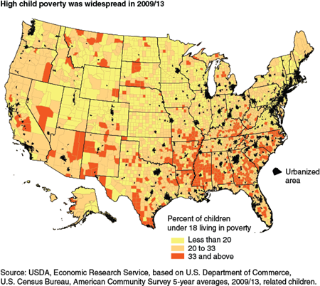
The problem of high and rising rural child poverty has been widespread but not pandemic across rural areas. Child poverty rates varied considerably across nonmetropolitan (rural) counties according to 2009 to 2013 county averages (county data on poverty are only available from the ACS for 5-year averages). One in five rural counties had child poverty rates of over 33 percent in 2009/13, but another one in five had child poverty rates of less than 16 percent. Overall, county average rates of child poverty rose from 20 percent to 25 percent over 1999-2009/13, with the proportion of counties with child poverty rates of over 33 percent doubling in this period. Meanwhile, estimated child poverty rates declined in one in five counties. To better understand this diversity of experience, we examine three factors shaping the geography of the change in rural child poverty over this period: changing economic conditions, young adult education, and family structure (see box, Measuring poverty).
The first factor, the economic conditions of the period, was most marked by the severe recession of 2007/09, but involved highly uneven impacts across rural areas and over time. After booming in the 1990s, rural manufacturing jobs began to disappear at the beginning of the 2000s, a trend that accelerated with the recession. While many local economies dependent on manufacturing had severe setbacks, other rural areas experienced booms in oil and gas mining with the expansion of fracking and other new extraction methods and never felt the recession. To understand the different effects of the recession across rural counties over this period, two measures reflecting changing labor market conditions were combined in this analysis: county change in number employed at least part of the year and county changes in earnings for people who were employed during the year (see box, Measuring Recession).
Parental education is another factor affecting child poverty. Job opportunities and earnings have generally declined over time for people with less education, especially for those without a high school diploma. In the 2013 ACS, the poverty rate for the population ages 25 and over without a high school diploma was 29 percent, nearly double the rate for those who had completed high school but gone no further (15 percent), and nearly 6 times the rate for college graduates (5 percent). While we do not have county data on the education of children’s parents, counties where low proportions of young adults (ages 25 to 44) have completed high school are likely to have more children in families with low educational attainment and higher child poverty levels. Young adult education varies considerably across rural counties. A quarter of rural counties had young adult dropout rates of 8 percent or lower, while one quarter had rates of 18 percent or above.
With respect to the third factor, family structure, single parents have difficulty simultaneously raising a family and earning enough to support the family. According to the 2013 ACS, the poverty rate for rural children in single-parent families was 50 percent, compared with 13 percent for children in rural married-couple families. The rise in poverty has been somewhat greater for children in single-parent families, for whom the child poverty rate was 43 percent in 1999, than it has been for children in married-couple families, for whom the rate was 10 percent in in 1999. This measure also shows considerable variation across rural counties, with one quarter of the counties having 25 percent or fewer children in single-parent households and a quarter having 38 percent or more children in this situation. The following analysis examines the role of these three factors in the geography of growth in child poverty over the study period.
Manufacturing Counties Severely Hit by the Recession Experienced a Substantial Rise in Child Poverty in 1999-2009/13
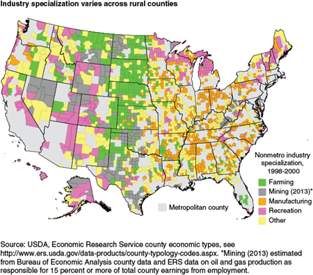
Nonmetropolitan counties have highly diverse industrial specializations. Where farming was once almost synonymous with rural, the predominance of farming as an industry in rural areas of the United States is now largely confined to the Plains States (see map). On average in 1998-2000, manufacturing predominated in many rural counties east of the Mississippi as well as in a scattering of counties further west. Manufacturing, a rural growth sector in the 1970s and 1990s, declined in both rural and urban areas in the 2000s. According to Bureau of Economic Analysis (BEA) data, the number of rural manufacturing jobs fell by 28 percent over 2001-10. There has been some subsequent recovery, but the number of rural manufacturing jobs was still 23 percent lower in 2013 than it had been in 2001. This is reflected in a decline in the number of manufacturing-dependent counties.
USDA’s Economic Research Service (ERS) classified counties as manufacturing-dependent in 1998-2000, based on whether average manufacturing earnings exceeded 25 percent of total earnings according to BEA county data. Applying the same threshold and data source (but a new 2001 industry classification system), the proportion of rural counties dependent on manufacturing dropped from 23 percent in 2001 to 13 percent in 2013.
Manufacturing has historically been a boon to rural low-skill workers, offering higher pay than other industries and often steadier work. But manufacturing was especially hard hit during the study period, and 43 percent of these counties had severe recession between 1999 and 2009/13, according to our index; only 6 percent avoided recession. The economic downturn in these counties was reflected in child poverty statistics. In 1999, manufacturing-dependent counties had average child poverty rates of 18 percent, 2 percentage points below the overall nonmetropolitan average. Their child poverty rates moved substantially upwards over the subsequent decade, reaching nearly 27 percent in 2009/13, a greater increase than observed in any other type of county.
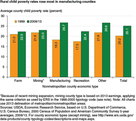
This experience stood in contrast to the trends for recreation counties, which are found in many mountain and coastal counties as well as forested counties across the northern Midwest and New England. While specialization in recreation is often considered to be associated with part-time, low-wage jobs, the average child poverty rate in recreation counties was actually below the nonmetropolitan county average in 1999. It remained so in 2009/13, even though a quarter of the rural recreational counties had severe recession as urban residents and potential retirees found themselves with less disposable income and fewer savings. With economic booms in both farming and mining, substantial proportions of both farming-dependent (47 percent) and mining-dependent (48 percent) counties were classified as having no recession (Because of the substantial increase in oil and gas mining, we applied the 1998-2000 criterion to 2013 data to define mining counties.) Despite this growth, however, neither type of county showed decline in their average child poverty rate.
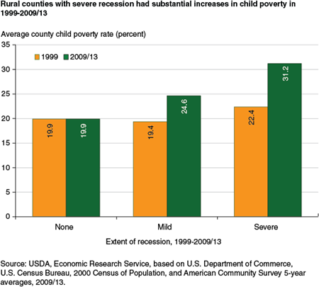
In general, rural counties with severe recession had much higher average child poverty rates in 2009/13 (31 percent) than they had in 1999 (22 percent). Counties largely immune from the recession, with growth in both employment and earnings, did not, however, have a corresponding decline in child poverty, which remained at 20 percent for the period. These results are consistent with the results for the generally prosperous farm and mining counties in suggesting that economic growth itself was largely unable to reduce child poverty over the past decade.
County Young Adult High School Completion Rates Are Strongly Related to Child Poverty
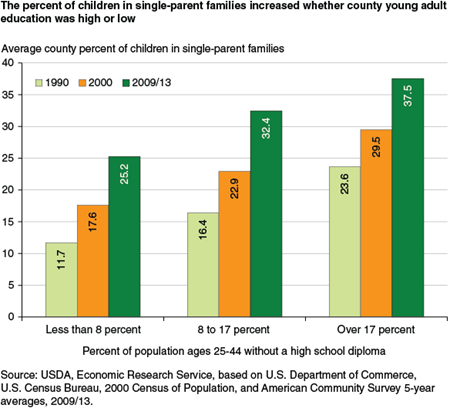
Young adult (ages 25-44) educational attainment improved considerably across rural counties over the 2000 to 2009/13 study period: the proportion of counties where 18 percent or more young adults (ages 25-44) lacked a high school diploma (or equivalent) fell from 43 percent to 25 percent. The proportion without a high-school diploma is a general indicator of low educational attainment, as counties with many non-high-school graduates among their young adults also tend to have high proportions with only a high school diploma, and lower proportions with a college degree.
County child poverty rates vary starkly with the proportion of young adults who have completed high school. Child poverty rates were generally higher in 2009/13 than they were in 1999, but at both times the average child poverty rate for counties with dropout rates of 18 percent or more was twice as high as the rate for counties with dropout rates of less than 8 percent.
Other things being equal, the improvements in educational attainment for young adults over the study period would have reduced county child poverty rates. To illustrate, if the average child poverty rates in the three county education categories had stayed at their 1999 levels, the shift in counties from higher to lower high school dropout categories would itself have meant a decline overall average county child poverty by 2 percentage points, to 18 percent. Clearly, other things were not equal, however, as the average rate instead rose by 5 percentage points between 1999 and 2009/13.
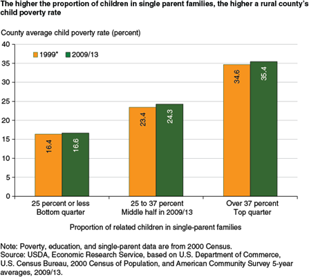
Where Rural County Proportions of Children in Single-Parent Families Went Up, So Did Child Poverty Rates
The overall proportion of rural children in single-parent rather than married-couple families rose markedly between 2000 and 2013, from 26 percent to 34 percent. Single-parent families have long been more prevalent in counties where young adult education is relatively low. However, over the past 2 decades, the county average percent of children in single-parent households has risen by about 14 percentage points regardless of the young adult high school dropout rate, and this rise was greater in the past decade than in the 1990s. In 2009/13, over a third of the children in the average low education county were living with a single parent, but that proportion was over 25 percent even for the quarter of rural counties with the lowest young adult high school dropout rates.
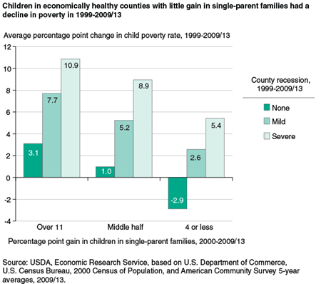
Only small increases in child poverty were observed over the 2000s in counties defined by percentage categories of children in single-parent families. However, a considerable number of counties shifted to higher percent-single-parent categories as the number of children in single-parent families rose. Thus, the number of nonmetropolitan counties with over 37 percent of their children in single-parent families rose from 192 in 2000 to 492, or a quarter of all rural counties, in 2009/13. These shifts alone would have raised overall average rural county child poverty rates by 4 percentage points, even if the poverty rates within each county category in the below chart had remained constant.
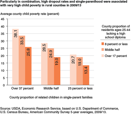
Differences in family structure are now more important than differences in educational attainment in explaining why some counties have higher child poverty rates than others. But the combination of high single-parent household rates with low high-school completion rates was particularly associated with high rates of child poverty in 2009/13.
There are several possible explanations for this finding. First, earnings depend on education, and young adults without a high school diploma are apt to find it especially difficult to support a family above the poverty line on a single salary. This difficulty likely increased over the past decade as earnings fell, particularly for the less schooled. Second, counties with the “most vulnerable” populations in 2000 (as defined by being in the top quarters in both the proportion of young adults without a high school diploma and the proportion of children in single-parent families) were highly prone to employment losses between 1999 and 2009/13. Some 47 percent of these counties, many of them manufacturing counties, had employment declines of at least 11 percent over this period. In contrast, fewer than 16 percent of the counties with the “least vulnerable” populations (those counties in the lowest quarter in both the high school dropout and single-parent family measures) had job losses this high.
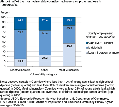
The third factor is that the population in the most vulnerable counties was apparently less able to adapt to employment decline, compared with the population in the least vulnerable counties. In general, employment change is accompanied by corresponding population change. However, vulnerable populations may be less mobile. Considering only counties with employment loss of 11 percent or more, the most vulnerable counties lost an average of 6 percent of their population between 2000 and 2011, but the least vulnerable counties lost considerably more, 11 percent. Where educational attainment levels are higher and people are not poor to begin with, it is easier for young adults to relocate and find jobs elsewhere.
The lack of outmigration likely put downward pressure on earnings in the most vulnerable counties, earnings already under pressure because of the general fall in earnings for low-skill workers. In the least vulnerable counties, employment loss of 11 percent or more was accompanied by enough loss in median earnings to create severe recessionary conditions, as measured by the composite index, in only 3 out of every 10 counties. In the most vulnerable counties, however, nearly 8 in 10 counties with this level of employment loss had severe recession. All told, 8 percent of the least vulnerable and 46 percent of the most vulnerable counties experienced severe recession. (The other counties fell in between, with 25 percent having severe recession.) As we saw earlier, severe recession was associated with substantial rises in poverty. Child poverty rates rose 10 percentage points, to an average of 42 percent in the most vulnerable counties experiencing severe recession.
The analysis thus far has focused on the interplay between initial county family and educational characteristics and the recession. We saw earlier that the increase in the proportion of children in single-parent families was also a factor in the rise in child poverty of the 1999-2009/13 period. When we graph changes in child poverty by county differences in the rise in single-parent children together with variation in recessionary influence, we find that counties with effectively no recession and little if any (4 percent or less) rise in single parenthood actually tended to experience a decline in child poverty over the period, of about 3 percentage points. In these 181 counties, as elsewhere, the proportion of young adult high school dropouts declined over the study period. In these counties, however, the benefits of improvements in education were not overwhelmed by the recession and/or a rise in single-parent families. More generally, the rise in children in single-parent families helps explain why the counties without recession did not generally have declining poverty. This chart is a lesson in the very diverse ways that broad national trends play out across rural areas.
Minority Counties Are More Vulnerable to Poverty, Largely Due to Differences in Educational Attainment and Family Structure
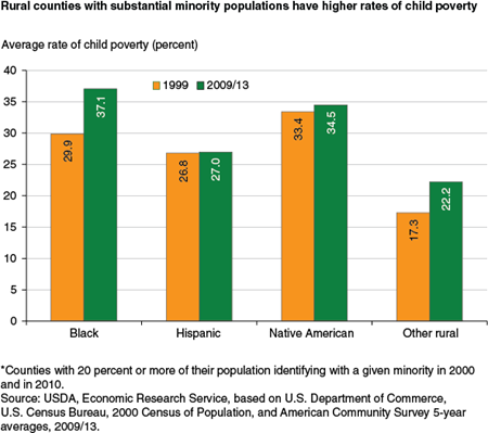
Poverty rates in Black, Hispanic, and Native American counties tended to be substantially higher than in other rural counties in 2009/13. These counties were defined in 2000 and 2010 by having at least 20 percent of their population comprised of the relevant minority.
To a large extent, differences across these county population types and between these and non-minority counties can be accounted for by differences in young adult high-school dropout rates, the prevalence of single-parent families and the degree to which these characteristics are found together. Thus, for instance, only 1 minority county out of 538 fits in the 2009/13 “least vulnerable” category described earlier, while 197 fit the “most vulnerable” category, comprising over 80 percent of its counties. In contrast, 241 of the nonminority counties are “least vulnerable,” while only 47 out of 1,433 nonminority counties fit the “most vulnerable” category.
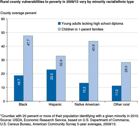
Vulnerabilities differ across the different types of minority county. Compared with nonminority counties, Black counties were higher in both the average proportion of young adults without high school diplomas and the average proportion of children living with only one parent, so much so that over half of the Black counties fit in the “most vulnerable” category in 2009/13. They comprised over half of the rural counties in that category.
Hispanic counties tended to be high in educational vulnerability, with many counties having elevated high-school dropout rates, but the proportion of children in single-parent families for this group was not far above the average for nonminority counties. Nonetheless, some Hispanic counties had relatively high proportions of children in single-parent families and 25 percent of the Hispanic counties fell into the “most vulnerable” category.
Native American counties generally had relatively low young adult high-school dropout rates in 2009/13. However, the average proportion of children in single-parent families was over a third. Some 16 percent of the Native American counties fell into the “most vulnerable” category.
While greater vulnerability helps explain the higher rates of child poverty in minority counties, it does not explain why only Black counties had a substantial rise in child poverty between 1999 and 2009/13. A large part of the answer appears to be that the Hispanic and Native American counties largely escaped the recession, with only 16 percent and 9 percent, respectively classified as severe recession counties. Black counties were hard hit, with 55 percent experiencing severe recession, over double the overall proportion. Many Hispanic and some Native American counties participated in the farming and mining booms noted earlier; few had manufacturing. Many Black counties, however, specialized in manufacturing, which as we saw earlier was associated with recession. Still manufacturing was not the whole story, as nearly half of the Black counties not classified as manufacturing counties had severe recession.
Three Questions to Answer…
The preceding analysis leaves several important questions unanswered. One question is whether the poor job opportunities that characterized at least the last 6 years in many rural counties may have contributed to the rise in single-parent households. Treating job growth and single parenthood as separate phenomena may understate the influence of the recession on family formation and stability and hence on child poverty. Economic stress may have undermined existing two-parent families and made the formation of new ones less attractive. Further research may help resolve this question.
A second question is the role of migration. This discussion may have wrongly left the impression that single-parent families are not mobile. The low rates of population decline in response to employment decline in the most vulnerable counties are striking. Nonetheless, previous research has showed that the poor do move, often in search of affordable housing as well as jobs. They may also move to areas where relevant services are more available. What further role migration may have played in producing the study results is a possible topic for future study.
A third question relates to the level at which influences are acting. Children in vulnerable families, with single parents who have not completed high school, generally have a high probability of being poor. This is a family-level influence. But children in vulnerable families may be much more likely to be poor in communities where a large proportion of children are in vulnerable families than where this vulnerability is rare. Research is beginning to suggest that families with few resources do better—are more likely to work, excel in school, and have healthy lifestyles—in middle class rather than low-income communities. This is a community-level influence. The county data used here does not allow us to separate the two levels. This, too, is a topic for future rural research.
Summary
The weak job market, with declining employment and earnings in most nonmetropolitan counties during 2000 to 2009/13, clearly played a role in the rise in child poverty over this period, particularly in counties with vulnerable children. Compounding the problem, the most vulnerable counties, often counties with substantial Black populations, were the ones most likely to experience severe recession.
The weak job market, however, was not the only important factor driving child poverty rates up. Also significant over this period was the rise in the proportion of children being raised in single-parent families. Changes in family structure, including declines in marriage rates and increases in divorce and cohabitation, perhaps influenced by the weak job market, was sufficient to account for much of the rise in county-average child poverty over the period. Educational attainment levels improved over the period but the positive effects of these changes on child poverty rates tended to be more than offset by the wide-spread increase in single-parent families. What we do not know from this analysis is the relative importance of community- versus family-level factors in shaping the relationships found in this study. To what extent, for instance, are children in single-parent, low-education families better off in communities where few other children are in this situation?
<a name='sidebar1'>Measuring poverty</a>
This analysis uses the official poverty measure as estimated in the Census Bureau’s American Community Survey (ACS) and Census 2000. The measure is based on self-reported household pre-tax income, adjusted for household size and, over time, increases in the cost of living. In 2013, the official poverty line was $23,624 for a family of four (two adults and two children). The official poverty measure does not take into account nonmonetary benefits, such as subsidized housing, food programs, and Medicare, or benefits from the Earned Income Tax Credit program. As these programs have grown over time, the official poverty measure has come somewhat less to reflect actual economic well-being and more to reflect well-being in the absence of these programs. The Census, in cooperation with other Federal agencies, has begun to develop and publish a “Supplemental Poverty Measure” (SPM) to take government programs—and area differences in cost of living—into account. However, the SPM is still somewhat experimental, and is not available in the ACS.
Two measures of child poverty are available from the ACS and earlier censuses. One measure considers the population under age 18 living in households where they are related to the household head, whether through family ties or by adoption. The other measure includes, in addition, individuals aged 15 through 17 who are living in their own households or with others to whom they are not related (e.g., foster children, children in communal housing). For this group, poverty is based on their own income or, if married, their joint income. The present analysis is based on the poverty of related children and results in slightly lower child poverty estimates than might be reported elsewhere.
<a name='sidebar2'>Measuring recession in individual counties</a>
To gauge the severity of the recession and other economic change over the study period, two measures were used: the number of people employed at all during the previous year and their median earnings. The information was drawn from the 2000 Census of Population and the ACS 5-year averages for 2009/13, the same sources used for the poverty statistics reported here. Governed by data availability, the period is much longer than the officially recognized recession, which in any case had a long recovery period. ERS calculated the percent changes in each of these measures, standardized the measures for nonmetropolitan counties so each had a zero average and a standard deviation of one, and summed them together to create a recession index. This method gives each measure equal weight in the index. As done with most of the measures in this study, the scale was divided into 3 parts based on the county ranking, so that a quarter of the counties fell into the lowest category, followed by a middle half, and a top quarter. For counties in the top quarter, employment went up an average of 11 percent over the period and inflation-adjusted earnings rose an average of over 5 percent. Although they may have had downturns over part of the study period, these counties are considered generally not to have experienced lasting effects of the recession. Counties in the middle half had average declines in employment and earnings of 4 and 5 percent, respectively, and are considered to have had mild recessions. Finally, the bottom quarter, labeled, “severe recession,” had an average employment decline of 13 percent and an average decline in median earnings of 15 percent. While these statistics suggest that the employment and earnings measures move in tandem, this is not always the case. Counties economically dependent on farming, for instance, tend to have had rising median earnings over this period, but declining employment.
Rural Economy & Population, USDA, Economic Research Service, November 2023
Rural America at a Glance, 2015 Edition, by Lorin Kusmin, USDA, Economic Research Service, November 2015
Rural Employment Trends in Recession and Recovery, by Thomas Hertz, Lorin Kusmin, Alexander Marré, and Timothy Parker, USDA, Economic Research Service, August 2014
Rural Child Poverty Chart Gallery, USDA, Economic Research Service, August 2019